Back to LUMEN-PS
Documentation · Photometric Stereo Pipeline

LUMEN-PS Documentation

Everything needed to run the pipeline: whether your scanner is suitable, what scans well, how the four captures become a material, how the solver repairs its own mistakes, and how to read the quality-assurance output it produces alongside every run.

How the method works

For a mostly matte surface, the brightness measured under light k is approximately Ik = ρ · max(N · Lk, 0), where ρ is the lighting-independent albedo, N is the unknown surface normal, and Lk is the calibrated light vector. Four rotations give four such equations per pixel. The solver estimates the three components of ρN, normalizes that vector to get N, and keeps its length as ρ.

Three observations is the mathematical minimum. The fourth is what makes the result trustworthy: it gives the solver room to reject one highlight or one shadow per pixel and still remain determined.

Capture

Four scans at 0°, 90°, 180°, and 270° with identical exposure and colour settings, captured through WIA 2.0 or supplied as lossless files.

Register

De-rotate, refine rigidly, then correct elastic settling with optical flow run on a lighting-invariant proxy rather than the raw pixels.

Solve

Fit the lamp azimuth and elevation, then solve the Lambertian system per pixel with outlier rejection and residual-guided repair.

Export & verify

Write normals, albedo, height, and alpha, then re-render all four inputs so the residuals show exactly where the model does and does not hold.
Quick Start

Windows app

  1. Install Python 3.11 or newer.
  2. Connect the scanner and install its WIA driver.
  3. Double-click run.bat.

The launcher creates an isolated virtual environment, installs dependencies, starts the local LUMEN-PS bench, and opens http://127.0.0.1:8756. From there: create a session, capture the four rotations, process, then drag the light around the interactive result. If an NVIDIA GPU is present, the first launch also installs a project-local CUDA runtime — a large one-time download, but no system-wide CUDA Toolkit is required.

Command line

python -m venv .venv
.venv\Scripts\Activate.ps1
pip install -r requirements.txt
# Optional NVIDIA CUDA backend:
pip install -r requirements-gpu.txt

python -m leafscan.cli capture --preview
python -m leafscan.cli capture --out scans\sample\k0.png --dpi 600 --color
# Rotate the subject 90 degrees and repeat for k1.png, k2.png, and k3.png.

python -m leafscan.cli run --scans scans\sample --out out

Two optional references improve the result. A blank scan of the same carrier card (flat.png) enables flat-field correction. Single-face corrugated cardboard scanned at 0° and 90° (calib0.png, calib90.png) lets the light elevation be fitted directly; without them, elevation is self-calibrated from re-rendering residuals.

Protect the platen

Use caution with any rigid object. A raised, heavy, sharp, or oversized subject can scratch or crack the scanner glass or damage the lid mechanism. Never press a rigid object down with the lid — use a disposable matte carrier card instead.

Will My Scanner Work?

The printer half of an all-in-one is irrelevant — LUMEN-PS needs a compatible flatbed. Verified hardware: an HP LaserJet Professional M1130/M1132 MFP over USB through WIA 2.0, at 75–1200 dpi. Other devices are expected to work when they meet the requirements below, but should pass the directional-light test first: scan the same subject at 0° and 90° and confirm the highlights shift.

RequirementNeededNotes
Windows driver exposed through WIA 2.0YesAutomatic capture is Windows/WIA. CLI processing can also run on suitable lossless scans captured another way.
Flatbed platenYesSheet-fed and ADF scanners cannot keep and rotate the subject on a common plane.
Directional, repeatable moving lampYesCIS units commonly have the useful lamp–sensor offset. Verify by comparing highlights between the 0° and 90° scans.
Manual or lockable brightness / contrast / colourStrongly recommendedAll four scans need identical processing. Disable auto exposure, auto colour, sharpening, and enhancement wherever the driver allows.
24-bit colour, lossless PNG or TIFFYesNever feed JPEG captures to the reconstruction. The tested WIA driver is 8-bit per channel, so sRGB is linearized in software.
600 dpi or higher optical resolutionRecommended1200 dpi captures fine relief; 600 dpi is faster and often sufficient.
Enough platen clearanceYesThe subject and fiducial card must lie flat without forcing the lid or loading the glass.

What Scans Well

The model assumes mostly diffuse reflection and shallow relief. Mild highlights are handled by outlier rejection; dominant reflections are not.

Good candidatesChallenging or unsupported
Leaves and pressed flowersPolished coins, foil, glossy plastic, wet surfaces
Paper, prints, cardboard, embossed stockTransparent or translucent objects with no diffuse surface
Fabric, leather, thin bark, flat natural texturesDeep objects that cast strong shadows or cannot stay registered
Shallow relief and mostly matte craft materialsAnything sharp, heavy, hot, dirty, or likely to damage the platen

The Pipeline

StageWhat happensWhy it matters
1 · CaptureScan at 0°, 90°, 180°, and 270° with identical exposure and colour settings.Produces four observations with different subject-relative light azimuths.
2 · LinearizeUndo the sRGB gamma and optionally divide by a blank-card flat field.Photometric stereo requires pixel values proportional to received light.
3 · RegisterDe-rotate using fiducials, refine the rigid alignment, then correct small elastic changes.The same output pixel must represent the same physical point in all four scans.
4 · CalibrateFit the lamp azimuth and elevation from a calibration card or from re-render error.The light elevation controls how strongly the recovered normals tilt.
5 · SolveRobustly solve I = ρ(N · L) per pixel, dropping highlight and shadow outliers.Separates the lighting-free albedo from the surface normal.
6 · RepairDetect inconsistent normals, identify the bad scan by leave-one-out re-solving, and inpaint only what is unrecoverable.Removes registration and gloss artifacts without smoothing away trustworthy vein relief.
7 · Integrate + verifyIntegrate the cleaned normal field into height, then re-render all four input views.Residual images show where the model explains — or fails to explain — the measurements.
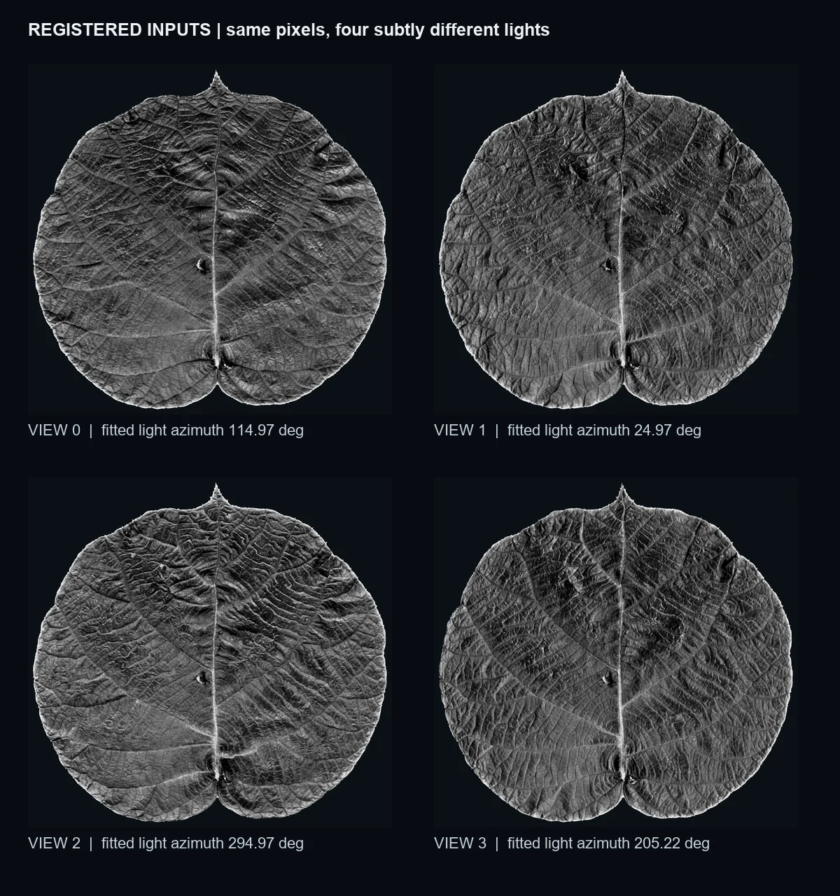
Four registered kiwi leaf luminance observations with their fitted light azimuths
The four captures after registration, each labelled with its fitted light azimuth. The tip, veins, and boundary now occupy identical pixels — only the illumination should differ.

Registration

The reconstruction is only as good as its registration. Any residual misalignment is interpreted by the solver as surface slope and becomes fake relief. Placing the four rotations onto one pixel grid is therefore its own small pipeline: rigid first, elastic second, with a per-pixel validity check at the end.

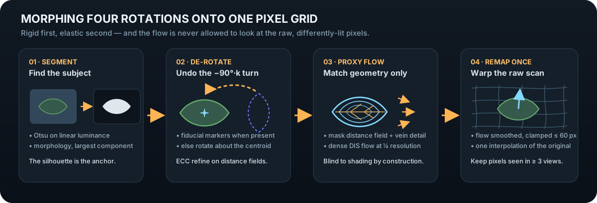
Registration pipeline diagram: segment the subject, de-rotate rigidly, estimate flow on a lighting-invariant proxy, then remap the raw scan once
Segment, de-rotate, estimate proxy flow, remap once.
  1. Segment. Otsu thresholding on linear luminance separates the darker subject from the bright platen, followed by morphological cleanup and a largest-component pass.
  2. De-rotate. Shared ArUco markers on a fiducial card give the rigid transform directly. Otherwise the scan is rotated by the nominal −90°·k about the subject's centroid and refined with ECC alignment — run on the masks' distance transforms rather than the images, so lighting cannot bias it.
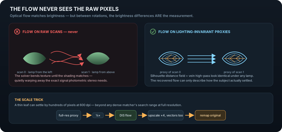
  3. Proxy flow. Dense DIS optical flow measures the elastic settling between rotations, computed on a lighting-invariant proxy rather than the raw pixels.
  4. Remap once. The flow field is smoothed, clamped to a sane maximum displacement, and applied to the full-detail original in a single interpolation. Pixels covered by fewer than three warped views are excluded from the solve as underdetermined.
Why the flow never sees the raw scans

Optical flow works by moving pixels until brightness matches — but between rotations, the brightness differences are the measurement. Run flow on the raw scans and it will happily bend the leaf until the shading agrees, silently erasing the very signal photometric stereo depends on. The proxy it sees instead is built from the silhouette's distance transform plus a high-pass of the luminance: both look identical no matter where the lamp sits, so the recovered flow can only describe how the subject physically settled.

Diagram contrasting optical flow on raw differently-lit scans against flow on lighting-invariant proxies
Flow is estimated at quarter scale — where hundreds of pixels of settling become dozens — then upscaled, with vector magnitudes scaled with it, before the single full-resolution remap.

Normal Repair

Even after registration, a flexible subject may settle a few pixels differently between rotations, and a glossy vein can violate the Lambertian model in a single observation. Either case pulls a solved normal sharply sideways. A generic blur would hide those pixels — and flatten genuine veins and creases along with them — so LUMEN-PS uses residual-guided selective repair instead.

Diagram of residual-guided normal filtering: detect, build trusted context, leave-one-out re-solve, and selectively merge
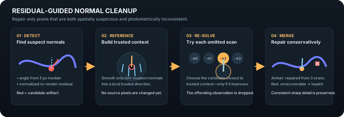
Detect, build trusted context, re-solve leaving one scan out, merge conservatively.
  1. Detect candidates. A pixel becomes suspect when its normal differs from the local 5 px component-median field, or when its albedo-normalized re-render residual is extreme. The residual test catches coherent artifact patches that would otherwise agree with their own local median.
  2. Build trusted context. Non-suspect neighbouring normals form a smooth reference direction. Empty support is filled with bounded, linear-time nearest-supported interpolation — there is no unbounded large-kernel blur.
  3. Identify the offending observation. For each suspect pixel the solver tries four leave-one-out candidates, and accepts the one closest to trusted context only when the angular agreement improves by the configured margin.
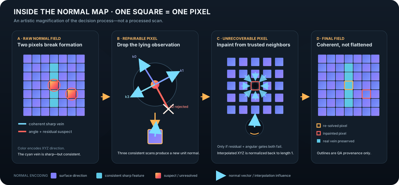
  4. Merge conservatively. A pixel that remains both far from trusted context and photometrically inconsistent is inpainted from its surroundings. A sharp but self-consistent normal is kept — sharpness alone is never enough to trigger replacement.
Pixel-level illustration of suspect normal detection, three-scan repair, selective inpainting, and the final coherent normal field
A repairable pixel still has three mutually consistent observations, so it is re-solved from real measurements. Only a pixel with no trustworthy three-view solution is interpolated from its neighbours and renormalized.
Filtered kiwi normal map beside its repair coverage map
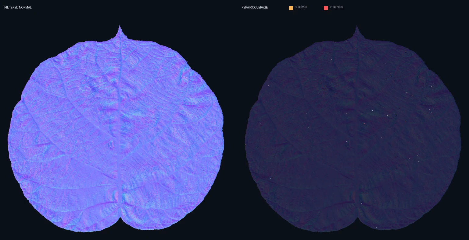
Repair coverage on the kiwi run. Amber marks pixels recovered from three consistent scans; red marks unrecoverable pixels that were selectively inpainted. Repair is sparse and targeted, not a whole-image smoothing pass.

Outputs

  • normal_gl.png and normal_dx.png — the recovered normal field in both conventions. Exported at 16-bit: the lamp–sensor baseline is small, so many recovered slopes differ by increments that would band in 8-bit.
  • Albedo — linear and sRGB, plus a ready-to-use RGBA pair with the alpha mask already composited.
  • height.png — 16-bit relief integrated from the cleaned normal field. Useful for displacement, but more sensitive to low-frequency drift than the normals it came from.
  • alpha.png — the subject mask derived during segmentation.
  • QA output — observed, predicted, and residual views for all four scans, mask agreement, rejection coverage, and misreg_repair.png, which records exactly which pixels were re-solved and which were inpainted.
  • Subsurface hint — for leaves, red light penetrates tissue more deeply than blue, so an R − B map is written for QA or shading experiments. It deliberately does not drive the normal solve.
Normals and height answer different questions

The normal map is the direct photometric result and preserves fine local slope. Height is obtained by integrating that slope field, which makes it useful for relief but more sensitive to low-frequency drift and boundary conditions. When the two disagree, trust the normals.

Performance & GPU

A 1200 dpi run can cover tens of millions of pixels, so LUMEN-PS uses a hybrid backend rather than forcing every operation onto one processor.

WorkloadBackend in auto modeOptimization
Photometric normal solveCPUFour binary sample weights produce at most 16 distinct 3×3 systems. Each is inverted once and applied to every matching pixel — no per-pixel matrix factorization.
RGB albedo recoveryCUDAProcesses VRAM-aware row tiles, avoiding a full four-view RGB stack allocation on the GPU.
QA re-render + residualsCUDAComputes predicted lighting and absolute residuals in bounded tiles.
Height integrationCUDARuns the Frankot–Chellappa FFT in float32 on the GPU; the CPU fallback also uses float32 to halve peak memory.
Alignment and optical flowCPU / OpenCVStays CPU-side to preserve the established interpolation behaviour. OpenCV is capped at four threads by default so the desktop stays responsive.
Misregistration cleanupHybridGrouped solves plus a bounded neighbourhood pass, with linear-time support filling instead of a widening blur.
runtime:
  compute: "auto"   # auto | cpu | gpu
  cpu_threads: 4    # OpenCV alignment thread cap

auto is recommended: it keeps the tiny grouped linear systems on the faster CPU path while sending large array and FFT workloads to CUDA. cpu disables CUDA entirely; gpu forces every supported operation onto CUDA and is mainly useful for profiling. GPU tiles are sized from currently free VRAM and cached allocations are released between stages, so a 4 GB laptop GPU works without starving the desktop. Both paths feed the same export code — acceleration never produces a different result.

Reading QA

Every run re-renders the recovered maps under each fitted scanner light and compares them against the original scans. The residual is the honest report card.

What you seeWhat it means
Low, noise-like residualThe model explains the scan. Trust is high — the filtered kiwi run sits at a mean residual of 0.0092–0.0099.
Bright veins or isolated sparklesSpecular leakage. Tighten outlier rejection.
Grey or white areas in misreg_repair.pngGrey was repaired by dropping one bad observation; white required selective inpainting.
A large smooth gradientFlat-field correction or light elevation is wrong.
Residual tracing the outlineRigid or non-rigid registration failed.
Fewer than three valid viewsThat pixel is underdetermined and excluded from the solve.
Mask agreement between the four registered scans
Mask agreement — how well the four silhouettes overlap after registration
Coverage map of observations rejected as highlight or shadow outliers
Rejection coverage — where observations were dropped as outliers
Subsurface hint map derived from the red minus blue channel difference
Subsurface hint — the R − B map, written for QA but never fed to the solve